Creating a Parametric Model

In this topic we discuss how you might develop SysML model elements for simulation (assuming existing knowledge of SysML modeling), configure these elements in the Configure SysML Simulation window, and observe the results of a simulation under some of the different definitions and modeling approaches. The points are illustrated by snapshots of diagrams and screens from the SysML Simulation examples provided in this chapter.

When creating a Parametric Model, you can apply one of three approaches to defining Constraint Equations:

Defining inline Constraint Equations on a Block element
Creating re-usable Constraint Blocks, and
Using connected constraint properties

You would also take into consideration:

Flows in physical interactions
Default Values and Initial Values
Simulation Functions
Value Allocation, and
Packages and Imports

Access

Ribbon

Simulate > SysMLSim > Manage > SysMLSim Configuration Manager

Defining inline Constraint Equations on a Block

Defining constraints directly in a Block is straightforward and is the easiest way to define constraint equations.

In this figure, constraint 'f = m * a' is defined in a Block element.

Tip: You can define multiple constraints in one Block.

Create a SysMLSim Configuration Artifact 'Force=Mass*Acceleration(1)' and point it to the Package 'FMA_Test'.
For 'FMA_Test', in the 'Value' column set 'SysMLSimModel'.
For Parts 'a', 'm' and 'f', in the 'Value' column set 'a' and 'm' to 'SimConstant' and (optionally) set 'f' to 'SimVariable'.
On the 'Simulation' tab, in the 'Properties to Plot' panel, select the checkbox against 'f'.
Click on the Solve button to run the simulation.

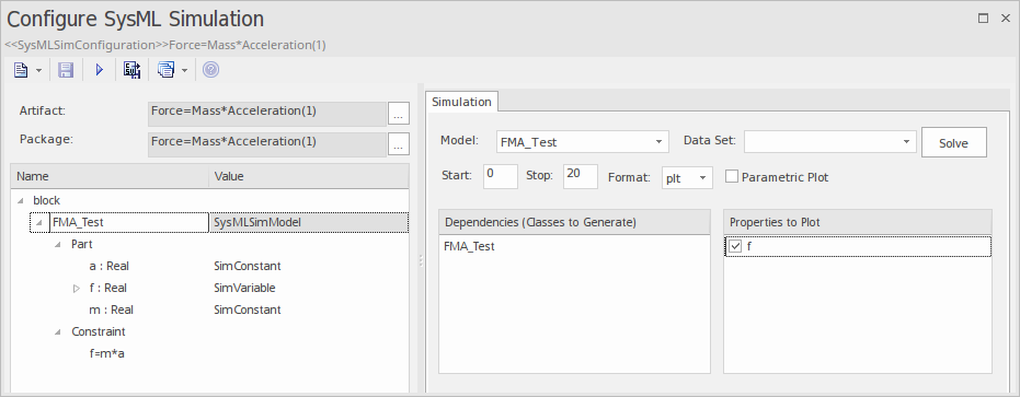
A chart should be plotted with f = 98.1 (which comes from 10 * 9.81).

Connected Constraint Properties

In SysML, constraint properties existing in Constraint Blocks can be used to provide greater flexibility in defining constraints.

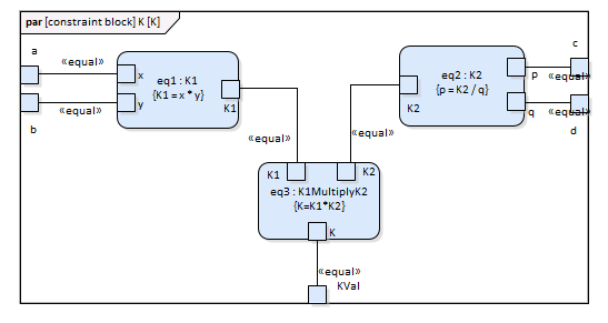
In this figure, Constraint Block 'K' defines parameters 'a', 'b', 'c', 'd' and 'KVal', and three constraint properties 'eq1', 'eq2' and 'eq3', typed to 'K1', 'K2' and 'K1MultiplyK2' respectively.

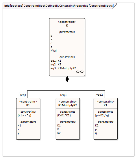
Create a Parametric diagram in Constraint Block 'K' and connect the parameters to the constraint properties with Binding connectors, as shown:

Create a model MyBlock with five Properties (Parts)
Create a constraint property 'eq' for MyBlock and show the parameters
Bind the properties to the parameters

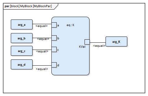
Provide values (arg_a = 2, arg_b = 3, arg_c = 4, arg_d = 5) in a data set
In the 'Configure SysML Simulation' dialog, set 'Model' to 'MyBlock' and 'Data Set' to 'DataSet_1'
In the 'Properties to Plot' panel, select the checkbox against 'arg_K'
Click on the Solve button to run the simulation

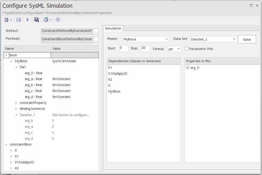
The result 120 (calculated as 2 * 3 * 4 * 5) will be computed and plotted. This is the same as when we do an expansion with pen and paper: K = K1 * K2 = (x*y) * (p*q), then bind with the values (2 * 3) * (4 * 5); we get 120.

What is interesting here is that we intentionally define K2's equation to be 'p = K2 / q' and this example still works.

We can easily solve K2 to be p * q in this example, but in some complex examples it is extremely hard to solve a variable from an equation; however, the Enterprise Architect SysMLSim can still get it right.

In summary, the example shows you how to define a Constraint Block with greater flexibility by constructing the constraint properties. Although we demonstrated only one layer down into the Constraint Block, this mechanism could work on complex models for an arbitrary level of use.

Creating Reuseable Constraint Blocks

If one equation is commonly used in many Blocks, a Constraint Block can be created for use as a constraint property in each Block. These are the changes we make, based on the previous example:

Create a Constraint Block element 'F_Formula' with three parameters 'a', 'm' and 'f', and a constraint 'f = m * a'

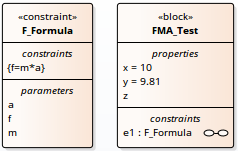
Tip: Primitive type 'Real' will be applied if property types are empty

Create a Block 'FMA_Test' with three properties 'x', 'y' and 'z', and give 'x' and 'y' the default values '10' and '9.81' respectively
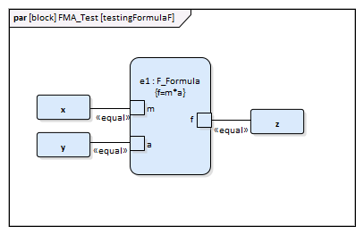
Create a Parametric diagram in 'FMA_Test', showing the properties 'x', 'y' and 'z'
Create a Constraint Property 'e1' typed to 'F_Formula' and show the parameters
Draw Binding connectors between 'x—m', 'y—a', and 'f—z' as shown:

Create a SysMLSimConfiguration Artifact element and configure it as shown in the dialog illustration:
     - In the 'Value' column, set 'FMA_Test' to 'SysMLSimModel'
     - In the 'Value' column, set 'x' and 'y' to 'SimConstant'
     - In the 'Properties to Plot' panel select the checkbox against 'Z'
     - Click on the Solve button to run the simulation

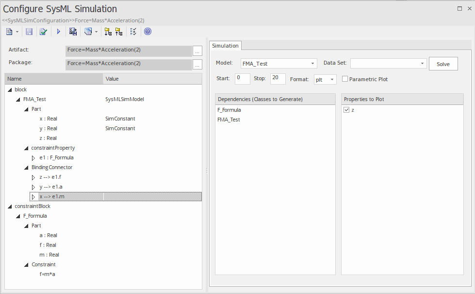
A chart should be plotted with f = 98.1 (which comes from 10 * 9.81).

Flows in Physical Interactions

When modeling for physical interaction, exchanges of conserved physical substances such as electrical current, force, torque and flow rate should be modeled as flows, and the flow variables should be set to the attribute 'isConserved'.

Two different types of coupling are established by connections, depending on whether the flow properties are potential (default) or flow (conserved):

Equality coupling, for potential (also called effort) properties
Sum-to-zero coupling, for flow (conserved) properties; for example, according to Kirchoff's Current Law in the electrical domain, conservation of charge makes all charge flows into a point sum to zero

In the generated Modelica code of the 'ElectricalCircuit' example:

connector ChargePort

flow Current i; //flow keyword will be generated if 'isConserved' = true

Voltage v;

end ChargePort;

model Circuit

Source source;

Resistor resistor;

Ground ground;

equation

connect(source.p, resistor.n);

connect(ground.p, source.n);

connect(resistor.p, source.n);

end Circuit;

Each connect equation is actually expanded to two equations (there are two properties defined in ChargePort), one for equality coupling, the other for sum-to-zero coupling:

source.p.v = resistor.n.v;

source.p.i + resistor.n.i = 0;

Default Value and Initial Values

If initial values are defined in SysML property elements ('Properties' dialog > 'Property' page > 'Initial' field), they can be loaded as the default value for a SimConstant or the initial value for a SimVariable.

In this Pendulum example, we have provided initial values for properties 'g', 'L', 'm', 'PI', 'x' and 'y', as seen on the left hand side of the figure. Since 'PI' (the mathematical constant), 'm' (mass of the Pendulum), 'g' (Gravity factor) and 'L' (Length of Pendulum) do not change during simulation, set them as 'SimConstant'.

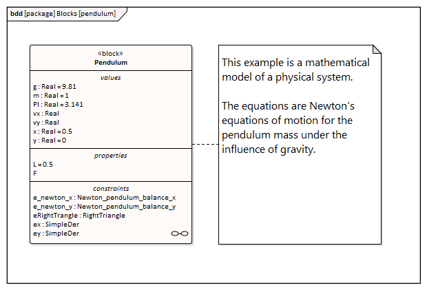
The generated modelica code resembles this:

class Pendulum

parameter Real PI = 3.141;

parameter Real m = 1;

parameter Real g = 9.81;

parameter Real L = 0.5;

Real F;

Real x (start=0.5);

Real y (start=0);

Real vx;

Real vy;

......

equation

......

end Pendulum;

Properties 'PI', 'm', 'g' and 'L' are constant, and are generated as a declaration equation

Properties 'x' and 'y' are variable; their starting values are 0.5 and 0 respectively, and the initial values are generated as modifications

Simulation Functions

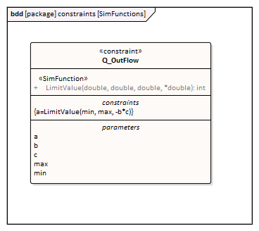
A Simulation function is a powerful tool for writing complex logic, and is easy to use for constraints. This section describes a function from the TankPI example.

In the Constraint Block 'Q_OutFlow', a function 'LimitValue' is defined and used in the constraint.

On a Block or Constraint Block, create an operation ('LimitValue' in this example) and open the 'Operations' tab of the Features window
Give the operation the stereotype 'SimFunction'
Define the parameters and set the direction to 'in/out'

Tips: Multiple parameters could be defined as 'out', and the caller retrieves the value in format of:

(out1, out2, out3) = function_name(in1, in2, in3, in4, ...); //Equation form

(out1, out2, out3) := function_name(in1, in2, in3, in4, ...); //Statement form

Define the function body in the text field of the 'Code' tab of the operation Properties window, as shown:

pLim :=
               if p > pMax then
                        pMax
              else if p < pMin then
                        pMin
              else
                        p;

When generating code, Enterprise Architect will collect all the operations stereotyped as 'SimFunction' defined in Constraint Blocks and Blocks, then generate code resembling this:

function LimitValue

input Real pMin;

input Real pMax;

input Real p;

output Real pLim;

algorithm

pLim :=

if p > pMax then

pMax

else if p < pMin then

pMin

else

end LimitValue;

Value Allocation

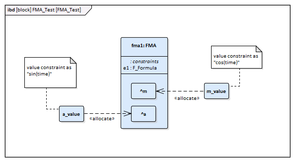
This figure shows a simple model called 'Force=Mass*Acceleration'.

A block 'FMA' is modeled with properties 'a', 'f', and 'm' and a constraintProperty 'e1', typed to Constraint Block 'F_Formula'
The block 'FMA' does not have any initial value set on its properties, and the properties 'a', 'f' and 'm' are all variable, so their value change depends on the environment in which they are simulated
Create a block 'FMA_Test' as a SysMLSimModel and add the property 'fma1' to test the behavior of block 'FMA'
Constraint 'a_value' to be 'sin(time)'
Constraint 'm_value' to be 'cos(time)'
Draw Allocation connectors to allocate values from environment to the model 'FMA'

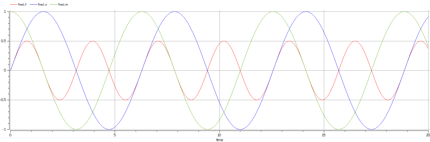
Select the 'Properties to Plot' checkboxes against 'fma1.a', 'fma1.m' and 'fma1.f'
Click on the Solve button to simulate the model

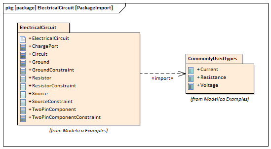
Packages and Imports

The SysMLSimConfiguration Artifact collects the elements (such as Blocks, Constraint Blocks and Value Types) of a Package. If the simulation depends on elements not owned by this Package, such as Reusable libraries, Enterprise Architect provides an Import connector between Package elements to meet this requirement.

In the Electrical Circuit example, the Artifact is configured to the Package 'ElectricalCircuit', which contains almost all of the elements needed for simulation. However, some properties are typed to value types such as 'Voltage', 'Current' and 'Resistance', which are commonly used in multiple SysML models and are therefore placed in a Package called 'CommonlyUsedTypes' outside the individual SysML models. If you import this Package using an Import connector, all the elements in the imported Package will appear in the SysMLSim Configuration Manager.

Learn more